Looking for a suitable motor?

小编
Published2025-10-15
The Fundamentals of Servo Motor Mathematical Modeling
Servo motors are at the heart of many modern systems, from robotics and CNC machines to automation in industries like aerospace and automotive. These motors excel because they provide high precision, excellent speed control, and are capable of executing a wide variety of motions. To fully harness their capabilities, engineers need to understand the mathematical models that govern servo motor performance.
In essence, the mathematical model of a servo motor helps us predict its behavior under different conditions. These models incorporate both the mechanical and electrical characteristics of the motor and the control systems that regulate it. The most common mathematical model for a servo motor is based on the following components:
The Mechanical Dynamics: Servo motors often control the motion of a mechanical load, such as a robotic arm or a conveyor belt. The relationship between the motor's output torque and the resulting motion of the load can be expressed using Newton’s laws of motion, particularly the second law, which relates torque to angular acceleration.
The Electrical Dynamics: Servo motors rely on electrical inputs to produce mechanical output. The electrical dynamics are described by Kirchhoff’s voltage law (KVL) and Ohm's law, which together explain how the input voltage is converted to current and, ultimately, the torque that the motor generates.
Feedback Control: One of the distinguishing features of a servo system is the feedback loop. This feedback loop monitors the actual position, velocity, or torque of the motor and compares it with the desired value (setpoint). Any error between the setpoint and actual value is corrected through the control system, often using techniques like PID (Proportional-Integral-Derivative) control.
Key Equations in Servo Motor Modeling
A basic servo motor system consists of two primary subsystems: the electrical system and the mechanical system. These subsystems are modeled using differential equations.
Electrical System Dynamics:
The electrical dynamics of a servo motor can be described by the following equation:
V(t) = L \frac{di(t)}{dt} + Ri(t) + K_e \omega(t)
( V(t) ) is the input voltage applied to the motor.
( L ) is the inductance of the motor windings.
( R ) is the resistance of the motor windings.
( i(t) ) is the current flowing through the motor windings.
( K_e ) is the back electromotive force (EMF) constant.
( \omega(t) ) is the angular velocity of the motor shaft.
This equation captures how the voltage input is related to the motor's current and speed, incorporating both the resistive and inductive effects of the motor windings.
Mechanical System Dynamics:
The mechanical dynamics are typically modeled using Newton’s second law for rotation:
J \frac{d\omega(t)}{dt} + B \omega(t) = T(t)
( J ) is the moment of inertia of the motor shaft and load.
( B ) is the damping coefficient (representing friction and other resistive forces).
( \omega(t) ) is the angular velocity.
( T(t) ) is the torque generated by the motor.
The motor generates torque in response to an electrical input, which causes the shaft to accelerate, overcoming the inertia of the system and any resistive forces like friction.
The Feedback Control System:
In a typical servo motor system, a controller constantly compares the desired position (setpoint) with the actual position and adjusts the motor input to minimize the error. This is often implemented using a PID controller, which has the general form:
u(t) = Kp e(t) + Ki \int e(t) dt + K_d \frac{de(t)}{dt}
( u(t) ) is the control input (voltage or current).
( e(t) ) is the error between the desired and actual output.
( Kp ), ( Ki ), and ( K_d ) are the proportional, integral, and derivative gains, respectively.
The PID controller plays a key role in maintaining the accuracy and stability of the system by continuously adjusting the motor’s input in response to any discrepancy between the desired and actual position or speed.
The Interplay Between Electrical and Mechanical Models
The key to understanding the servo motor’s operation lies in the interaction between the electrical and mechanical models. The electrical system provides the torque, which, in turn, drives the mechanical system. The feedback loop continuously adjusts the input voltage to minimize the position or speed error, ensuring that the motor operates with high precision.
In practice, this means that when an error is detected, the controller will adjust the motor input to reduce the difference between the desired and actual output. This results in a dynamic system that can quickly respond to changes in load, speed, or position, making servo motors ideal for tasks requiring high accuracy and rapid response times.
Advanced Concepts and Applications of Servo Motor Models
While the basic servo motor model provides a solid foundation, real-world applications often require more advanced techniques to handle the complexities of the system. This section will explore some of these advanced concepts, including the use of state-space models, nonlinear dynamics, and optimization methods to improve performance.
State-Space Modeling of Servo Motors
In many cases, it’s more practical to represent the servo motor system in state-space form, which allows for a more systematic analysis and easier implementation in digital control systems. State-space models represent the system using a set of first-order differential equations rather than second-order equations.
A typical state-space model for a servo motor consists of a set of equations describing both the electrical and mechanical subsystems. The state variables can include the motor’s angular position, velocity, and current, along with their derivatives. The general form of the state-space model is:
\dot{x}(t) = Ax(t) + Bu(t)
( x(t) ) is the state vector (e.g., position, velocity, current).
( u(t) ) is the input vector (e.g., voltage).
( y(t) ) is the output vector (e.g., position or velocity).
( A ), ( B ), ( C ), and ( D ) are matrices that describe the system dynamics.
State-space models provide a compact and efficient way to model the system, making them ideal for use in modern control algorithms, such as optimal control or model predictive control.
Nonlinearities and Practical Considerations
While the basic servo motor model assumes linear behavior, real-world motors often exhibit nonlinear characteristics due to factors like friction, saturation, and hysteresis. These nonlinearities can affect the performance of the motor, particularly in systems requiring high precision.
To account for nonlinearities, more sophisticated techniques like linearization or feedback linearization are often employed. These methods involve approximating the nonlinear system with a linear model near the operating point or using nonlinear control strategies to maintain stability and performance.
Additionally, practical considerations such as power supply limitations, motor heating, and mechanical wear-and-tear need to be factored into the model. These factors can introduce additional complexity, but they can also be mitigated using advanced techniques such as adaptive control or system identification.
Optimization for Improved Performance
The final piece of the puzzle lies in optimizing the servo motor system for specific applications. The performance of a servo motor can be enhanced through techniques such as parameter tuning of the PID controller, model predictive control, or genetic algorithms. Optimization methods can improve factors like energy efficiency, response time, and robustness in the face of disturbances.
For example, model predictive control (MPC) uses an explicit model of the system to predict future behavior and optimize control inputs over a finite time horizon. By solving an optimization problem at each time step, MPC can provide superior performance compared to traditional control methods.
Real-World Applications of Servo Motor Models
Servo motors are used in a vast array of applications where precision is critical. In robotics, servo motors enable precise control of limbs and joints, allowing for tasks like picking up objects or navigating difficult terrain. In CNC machines, servo motors drive the movement of cutting tools with high precision, ensuring that parts are manufactured to exact specifications. In the aerospace industry, servo motors control the position of flight control surfaces, ensuring stable and accurate flight.
By leveraging the power of mathematical modeling, engineers can design servo motor systems that are not only highly efficient but also adaptable to changing conditions and diverse applications.
In conclusion, the mathematical modeling of servo motors is an essential tool for understanding and optimizing their performance. By incorporating both electrical and mechanical dynamics, along with feedback control systems, engineers can create highly responsive and precise systems. With advanced techniques like state-space modeling, nonlinear control, and optimization, the potential for improving servo motor performance is limitless. Whether you're designing a robotic arm or optimizing a CNC machine, understanding the servo motor mathematical model is key to unlocking the full potential of these powerful components.
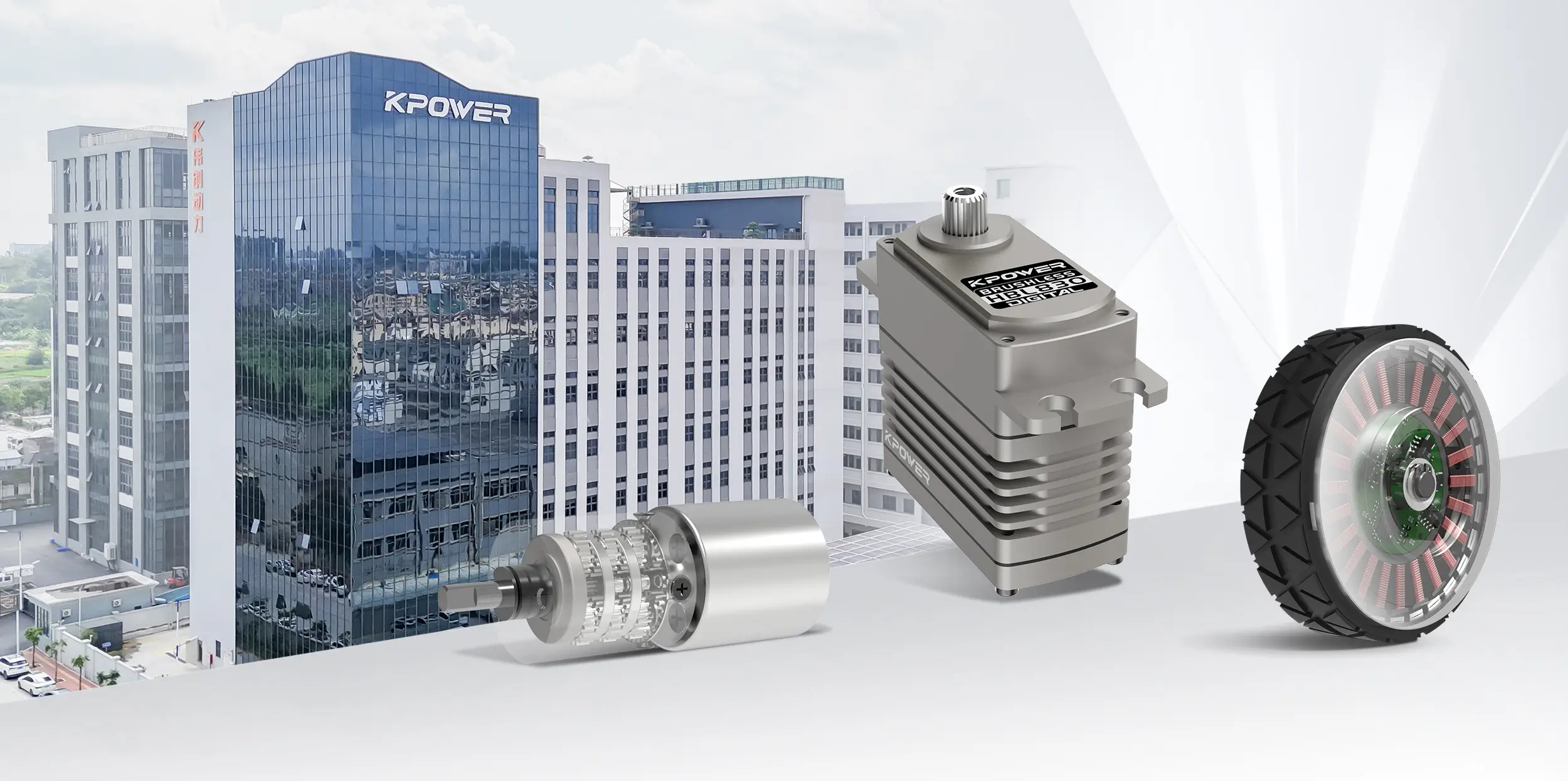
Leveraging innovations in modular drive technology, Kpower integrates high-performance motors, precision reducers, and multi-protocol control systems to provide efficient and customized smart drive system solutions.
Update:2025-10-15
Contact Kpower's product specialist to recommend suitable motor or gearbox for your product.